2.2.1. Anti-Aliasing¶

Because downsampling is the process of reducing a signal sampling frequency, it can cause severe aliasing by breaking the Shannon criteria.

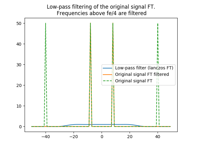
Hence, it is highly advised to provide Sirius a low-pass filter to apply to the original signal spectrum before downsampling it. Once the high frequencies are filtered, Sirius can safely decimate the original signal.

Such a low-pass filter must cut-off the frequencies $f, |f| > |\frac{f_e}{2*z_d}|$ with $z_d$ the downsampling factor.

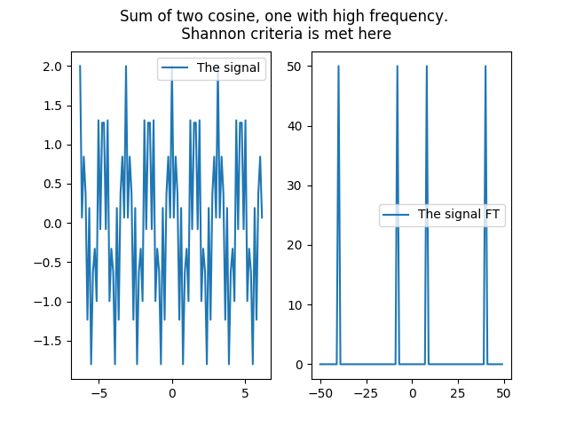
Here is an example based on a high frequency cosine to emphasize the potential aliasing when downsampling :

# cosine signal based on two cosine, one with high frequency
In [1]: x,cos4 = create_1D_cosine( 100, 4)

In [2]: x,cos20 = create_1D_cosine( 100, 20)

In [3]: s = cos4+cos20

In [4]: fft_s = np.fft.fftshift(np.fft.fft(s))

In [5]: plt.suptitle('Sum of two cosine, one with high frequency.\n Shannon criteria is met here');

In [6]: plt.subplot(121);

In [7]: plt.plot(x, s, label='The signal');plt.legend();

In [8]: plt.subplot(122);

In [9]: plt.plot(np.fft.fftshift(np.fft.fftfreq(fft_s.size))*fft_s.size, fft_s, label='The signal FT');plt.legend();

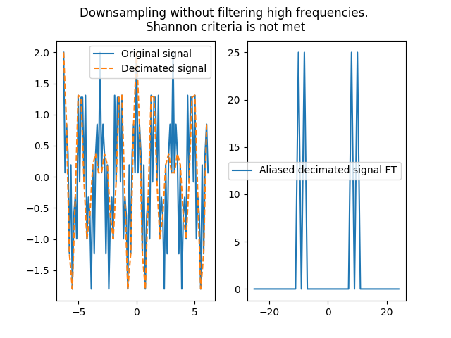
# decimating the signal without caution
In [10]: s_decim = s[0::2]

In [11]: plt.close()

In [12]: plt.suptitle('Downsampling without filtering high frequencies. \nShannon criteria is not met');

In [13]: plt.subplot(121);

In [14]: plt.plot(x,s,label='Original signal');

In [15]: plt.plot(x[::2],s_decim,'--', label='Decimated signal');plt.legend()
Out[15]: <matplotlib.legend.Legend at 0x7f63f94d7f90>

In [16]: plt.subplot(122);

In [17]: plt.plot(np.fft.fftshift(np.fft.fftfreq(s_decim.size))*s_decim.size, np.fft.fftshift(np.fft.fft(s_decim)), label='Aliased decimated signal FT');plt.legend()
Out[17]: <matplotlib.legend.Legend at 0x7f63f94f9e10>

../_images/hig_freq_cosine_decimated_aliasing.png

# decimating after low-pass filtering
In [18]: x_, lanczos_kernel_up2 = create_1D_lanczos( 50, a=5, step=2)

In [19]: lanczos_kernel_up2[0::2]/=(np.sum(lanczos_kernel_up2[0::2])/0.5)

In [20]: lanczos_kernel_up2[1::2]/=(np.sum(lanczos_kernel_up2[1::2])/0.5)

In [21]: fft_lanczos = np.fft.fftshift(np.fft.fft(np.fft.ifftshift(lanczos_kernel_up2[0:-1])))

In [22]: plt.close()

In [23]: plt.title('Low-pass filtering of the original signal FT.\n Frequencies above fe/4 are filtered')
Out[23]: Text(0.5,1,'Low-pass filtering of the original signal FT.\n Frequencies above fe/4 are filtered')

In [24]: plt.plot(np.fft.fftshift(np.fft.fftfreq(fft_s.size))*fft_s.size, fft_lanczos, label='Low-pass filter (lanczos FT)');plt.legend()
Out[24]: <matplotlib.legend.Legend at 0x7f63fb570090>

In [25]: plt.plot(np.fft.fftshift(np.fft.fftfreq(fft_s.size))*fft_s.size, fft_s * fft_lanczos, label='Original signal FT filtered'); plt.legend()
Out[25]: <matplotlib.legend.Legend at 0x7f63fb5df4d0>

In [26]: plt.plot(np.fft.fftshift(np.fft.fftfreq(fft_s.size))*fft_s.size, fft_s, '--', label='Original signal FT');plt.legend()
Out[26]: <matplotlib.legend.Legend at 0x7f63fb570b90>

In [27]: s_filtered = np.fft.ifft(np.fft.ifftshift(fft_s * fft_lanczos))

In [28]: s_filtered_decim = s_filtered[0::2]

In [29]: plt.close()

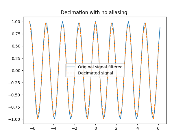
In [30]: plt.title('Decimation with no aliasing.')
Out[30]: Text(0.5,1,'Decimation with no aliasing.')

In [31]: plt.plot(x, s_filtered, label='Original signal filtered');

In [32]: plt.plot(x[::2],s_filtered_decim,'--', label='Decimated signal');plt.legend()
Out[32]: <matplotlib.legend.Legend at 0x7f63fb618710>

../_images/hig_freq_cosine_decimated_no_aliasing.png

In [33]: plt.close()

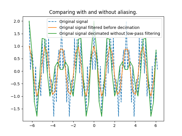
In [34]: plt.title('Comparing with and without aliasing.')
Out[34]: Text(0.5,1,'Comparing with and without aliasing.')

In [35]: plt.plot(x,s,'--',label='Original signal');

In [36]: plt.plot(x[::2],s_filtered_decim,label='Orignal signal filtered before decimation');

In [37]: plt.plot(x[::2],s_decim, label='Orignal signal decimated without low-pass filtering'); plt.legend()
Out[37]: <matplotlib.legend.Legend at 0x7f63fbe76750>