2.1.2. Tile processing of the large image:
2.1.2.1. The implicit edges discontinuities and their associated artifacts
In order to process satellite images, Sirius divides it in tiles (blocks). Those tiles are then executed independently from each other.
Though there is no particular reason for a natural signal / image to be periodic, Fourier Transform implicitly assumes it is. This leaves us with a periodized signal / image with probably strong discontinuities across its edges. This involves artifacts in the frequency domain that penalises the resampling process.
The tiling process that divides the images with arbitrary borders can only emphasized those artifacts.
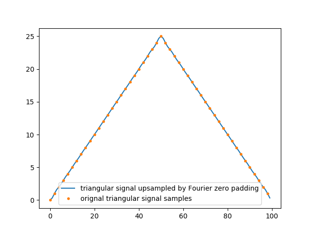
Below is an example with a triangular 1D signal (periodic) and a linear signal (half the triangle) with strong edges discontinuities. Both signals are zero padded :
In [1]: n=50

In [2]: z=2

In [3]: tri = create_1D_triangle_signal(n)

In [4]: tri_zpd = zoom_freq_zpd( tri, zoom_factor=z)

In [5]: plt.plot(tri_zpd, label='triangular signal upsampled by Fourier zero padding');

In [6]: plt.plot(np.arange(0,n*z,z),tri,'.',label='orignal triangular signal samples');plt.legend()
Out[6]: <matplotlib.legend.Legend at 0x7f63f8f488d0>

In [7]: plt.close()

In [8]: halftri = create_1D_ramp(n)

In [9]: halftri_zpd = zoom_freq_zpd( halftri, zoom_factor=z)

In [10]: plt.plot(halftri_zpd, label='ramp signal upsampled by Fourier zero padding');

In [11]: plt.plot(np.arange(0,n*z,z), halftri,'.',label='orignal ramp signal samples');plt.legend()
Out[11]: <matplotlib.legend.Legend at 0x7f63f8e4d950>
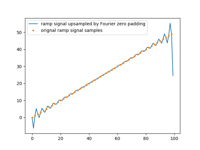
Those artifacts come from the fact that only a finite number of terms of the Fourier series can actually be used for numerical processing. Then, even though their limits do not overshoot the signal and will allow for a discontinuous signal to be approximated by infinite series of continuous sinusoids, every partial Fourier series can overshoot it. And it can actually be shown that the overshoot near a discontinuity will always be about 9% ([Hewitt & Hewitt, 1979]).
2.1.2.2. The possible solutions
2.1.2.2.1. Margin the original data
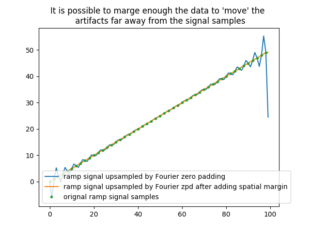
One way to get rid of these artifacts is to marge the original data by propagating the first and the last value of the signal, before and after it.
In [12]: marge_factor=4

In [13]: halftri_zpd_spatially = zero_pad(halftri, marge_factor)

In [14]: halftri_zpd_spatially[halftri_zpd_spatially.size/2+halftri.size/2:halftri_zpd_spatially.size] = halftri[-1]

In [15]: halftri_zpd_spatially_zpd = zoom_freq_zpd( halftri_zpd_spatially, zoom_factor=z)

In [16]: plt.title('It is possible to marge enough the data to \'move\' the \n artifacts far away from the signal samples');

In [17]: plt.plot(halftri_zpd, label='ramp signal upsampled by Fourier zero padding');

In [18]: plt.plot(halftri_zpd_spatially_zpd[halftri.size*(marge_factor-1)*z/2:halftri.size*(marge_factor-1)*z/2+halftri_zpd.size], label='ramp signal upsampled by Fourier zpd after adding spatial margin');

In [19]: plt.plot(np.arange(0,n*z,z), halftri,'.',label='orignal ramp signal samples');plt.legend()
Out[19]: <matplotlib.legend.Legend at 0x7f63f8cfb3d0>
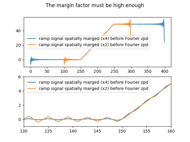
Note that the margin factor must be high enough :
In [20]: marge_factor=2

In [21]: halftri_zpd_spatially_mf2 = zero_pad(halftri, marge_factor)

In [22]: halftri_zpd_spatially_mf2[halftri_zpd_spatially_mf2.size/2+halftri.size/2:halftri_zpd_spatially_mf2.size] = halftri[-1]

In [23]: halftri_zpd_spatially_mf2_zpd = zoom_freq_zpd( halftri_zpd_spatially_mf2, zoom_factor=z)

In [24]: plt.suptitle('The margin factor must be high enough');

In [25]: plt.subplot(211)
Out[25]: <matplotlib.axes._subplots.AxesSubplot at 0x7f63f8d18b10>

In [26]: plt.plot(halftri_zpd_spatially_zpd, label='ramp signal spatially marged (x4) before Fourier zpd');plt.legend();

In [27]: plt.plot(np.arange(100, 100+halftri_zpd_spatially_mf2_zpd.size), halftri_zpd_spatially_mf2_zpd, label='ramp signal spatially marged (x2) before Fourier zpd');plt.legend();

In [28]: plt.subplot(212)
Out[28]: <matplotlib.axes._subplots.AxesSubplot at 0x7f63f8cd0910>

In [29]: plt.plot(halftri_zpd_spatially_zpd, label='ramp signal spatially marged (x4) before Fourier zpd');plt.legend();

In [30]: plt.plot(np.arange(100, 100+halftri_zpd_spatially_mf2_zpd.size), halftri_zpd_spatially_mf2_zpd, label='ramp signal spatially marged (x2) before Fourier zpd');plt.legend();

In [31]: plt.xlim(130,160)
Out[31]: (130, 160)

In [32]: plt.ylim(-1,6)
Out[32]: (-1, 6)
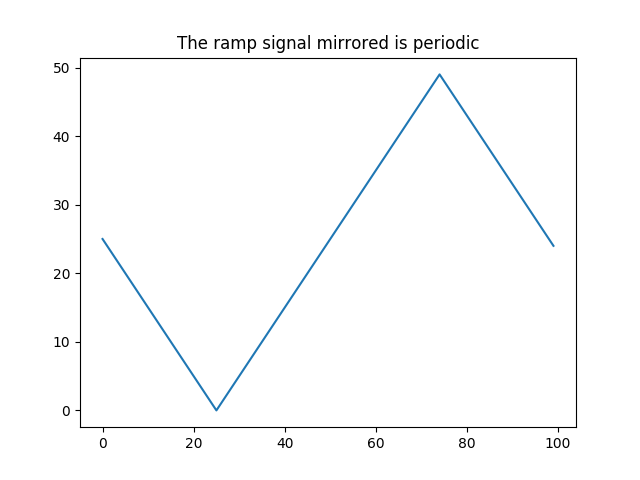
2.1.2.2.2. Mirroring the original data
One other way to look at it is to simply suppress the discontinuity by mirroring the signal.
In [33]: marge_factor=2
In [34]: halftri_mirrored = mirror(halftri, margin_factor=marge_factor)
In [35]: halftri_mirrored_zpd = zoom_freq_zpd( halftri_mirrored, zoom_factor=z)
In [36]: plt.title('The ramp signal mirrored is periodic');
In [37]: plt.plot(halftri_mirrored, label='mirrored ramp signal');
In [38]: plt.close()
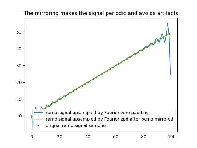
In [39]: plt.title('The mirroring makes the signal periodic and avoids artifacts');
In [40]: plt.plot(halftri_zpd, label='ramp signal upsampled by Fourier zero padding');
In [41]: plt.plot(halftri_mirrored_zpd[halftri.size*(marge_factor-1)*z/2:halftri.size*(marge_factor-1)*z/2+halftri_zpd.size], label='ramp signal upsampled by Fourier zpd after being mirrored');
In [42]: plt.plot(np.arange(0,n*z,z), halftri,'.',label='orignal ramp signal samples');plt.legend()
Out[42]: <matplotlib.legend.Legend at 0x7f63f8c17990>
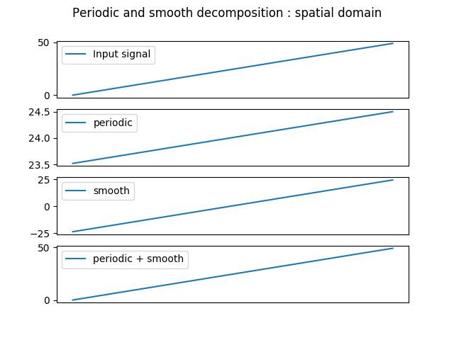
2.1.2.2.3. The periodic + smooth decomposition
The two previous methods implies adding ‘fake’ samples to the input data, which might be very time consuming if done for every tile of a satellite image. The solution proposed by [Moisan, 2011] however can deal with discontinuous signal with only a little overhead. It consists in decomposing the input signal into two sub-signals, one being periodic, and the other being smooth. The periodic signal can then be upsampled in Fourier domain without concerns about the artifacts discussed in this chapter. The smooth one, built from the differences located at the data edges, is upsampled spatially with a simple bilinear filter.
In [43]: n = halftri.size
#1 : Compute smooth part
In [44]: x = np.arange(n)
In [45]: s = np.zeros(halftri.shape)
In [46]: s = ((halftri[n-1] - halftri[0])/np.float(n)) * (x - (n-1)/2)
# 2 : Compute periodic part
In [47]: p = halftri - s
# 3 : Zero padds the periodic part
In [48]: tf_p = np.fft.fft(p)
In [49]: z_tf_p = fft1D_zero_pad(tf_p, zoom_factor=2)
# 4 : Interpolate the smooth part spatially with a blinear interpolator
In [50]: bln_interp_s = interp1d(s, zoom_factor=2)
# 5 : Merged p & s zoomed and FT-1
In [51]: halftri_p_fzpd_and_s_bln = np.fft.ifft(z_tf_p) + bln_interp_s
# plot the decomposition
In [52]: plt.suptitle('Periodic and smooth decomposition : spatial domain')
Out[52]: Text(0.5,0.98,'Periodic and smooth decomposition : spatial domain')
In [53]: plt.subplot(411)
Out[53]: <matplotlib.axes._subplots.AxesSubplot at 0x7f63f8c179d0>
In [54]: plt.plot(halftri, label='Input signal')
Out[54]: [<matplotlib.lines.Line2D at 0x7f63f8a59490>]
In [55]: plt.legend()
Out[55]: <matplotlib.legend.Legend at 0x7f63f8a59350>
In [56]: plt.tick_params(axis='x', which='both', bottom=False, top=False, labelbottom=False)
In [57]: plt.subplot(412)
Out[57]: <matplotlib.axes._subplots.AxesSubplot at 0x7f63f8a651d0>
In [58]: plt.plot(p, label='periodic')
Out[58]: [<matplotlib.lines.Line2D at 0x7f63f8a1c150>]
In [59]: plt.legend()
Out[59]: <matplotlib.legend.Legend at 0x7f63f8c8c710>
In [60]: plt.tick_params(axis='x', which='both', bottom=False, top=False, labelbottom=False)
In [61]: plt.subplot(413)
Out[61]: <matplotlib.axes._subplots.AxesSubplot at 0x7f63f8a25050>
In [62]: plt.plot(s, label='smooth')
Out[62]: [<matplotlib.lines.Line2D at 0x7f63f89da210>]
In [63]: plt.legend()
Out[63]: <matplotlib.legend.Legend at 0x7f63f89da0d0>
In [64]: plt.tick_params(axis='x', which='both', bottom=False, top=False, labelbottom=False)
In [65]: plt.subplot(414)
Out[65]: <matplotlib.axes._subplots.AxesSubplot at 0x7f63f89da110>
In [66]: plt.plot(p+s, label='periodic + smooth')
Out[66]: [<matplotlib.lines.Line2D at 0x7f63f897fe50>]
In [67]: plt.legend()
Out[67]: <matplotlib.legend.Legend at 0x7f63f897fd10>
In [68]: plt.tick_params(axis='x', which='both', bottom=False, top=False, labelbottom=False)
In [69]: plt.close()
# plot the result
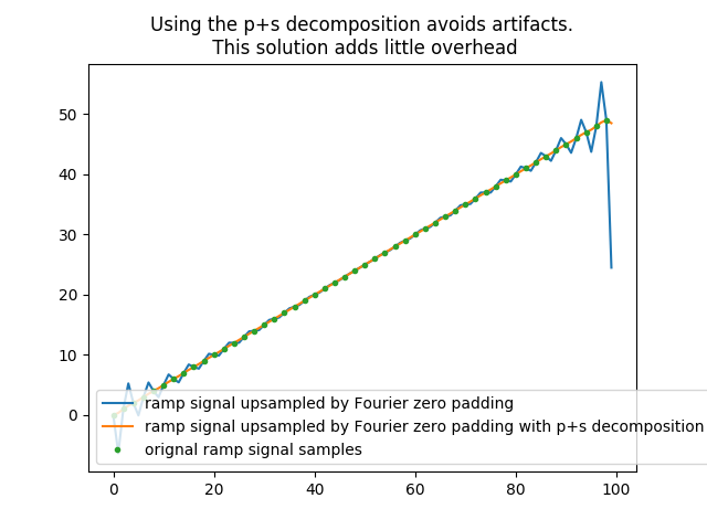
In [70]: plt.title('Using the p+s decomposition avoids artifacts.\n This solution adds little overhead');
In [71]: plt.plot(halftri_zpd, label='ramp signal upsampled by Fourier zero padding');
In [72]: plt.plot(halftri_p_fzpd_and_s_bln, label='ramp signal upsampled by Fourier zero padding with p+s decomposition');
In [73]: plt.plot(np.arange(0,n*z,z), halftri,'.',label='orignal ramp signal samples');plt.legend()
Out[73]: <matplotlib.legend.Legend at 0x7f63f88bd110>
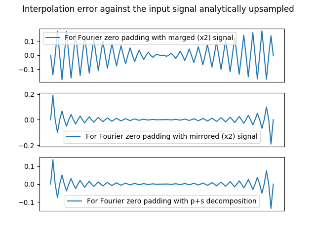
2.1.2.3. Conclusion : Sirius uses the p+s decomposition
Because it adds little overhead the p+s decomposition is the solution processed by Sirius to Fourier Transform each tile.
Below is a little comparison of the three methods presented above :
In [74]: halftri_analytically_zoomed = create_1D_ramp(50, step=2)[0:50*2-1]

In [75]: plt.suptitle('Interpolation error against the input signal analytically upsampled')
Out[75]: Text(0.5,0.98,'Interpolation error against the input signal analytically upsampled')

In [76]: plt.subplot(311)
Out[76]: <matplotlib.axes._subplots.AxesSubplot at 0x7f63f88e8310>

In [77]: marge_factor = 2

In [78]: plt.plot(halftri_analytically_zoomed-halftri_zpd_spatially_mf2_zpd[halftri.size*(marge_factor-1)*z/2:halftri.size*(marge_factor-1)*z/2+halftri_zpd.size-1], label='For Fourier zero padding with marged (x2) signal')
Out[78]: [<matplotlib.lines.Line2D at 0x7f63f8770b90>]

In [79]: plt.legend()
Out[79]: <matplotlib.legend.Legend at 0x7f63f8770a90>

In [80]: plt.tick_params(axis='x', which='both', bottom=False, top=False, labelbottom=False)

In [81]: plt.subplot(312)
Out[81]: <matplotlib.axes._subplots.AxesSubplot at 0x7f63f877a1d0>

In [82]: plt.plot(halftri_analytically_zoomed-halftri_mirrored_zpd[halftri.size*(marge_factor-1)*z/2:halftri.size*(marge_factor-1)*z/2+halftri_zpd.size-1], label='For Fourier zero padding with mirrored (x2) signal')
Out[82]: [<matplotlib.lines.Line2D at 0x7f63f8732950>]

In [83]: plt.legend()
Out[83]: <matplotlib.legend.Legend at 0x7f63f8732850>

In [84]: plt.tick_params(axis='x', which='both', bottom=False, top=False, labelbottom=False)

In [85]: plt.subplot(313)
Out[85]: <matplotlib.axes._subplots.AxesSubplot at 0x7f63f873b0d0>

In [86]: plt.plot(halftri_analytically_zoomed-halftri_p_fzpd_and_s_bln[0:50*2-1], label='For Fourier zero padding with p+s decomposition')
Out[86]: [<matplotlib.lines.Line2D at 0x7f63f86f1550>]

In [87]: plt.legend()
Out[87]: <matplotlib.legend.Legend at 0x7f63f86f1450>

In [88]: plt.tick_params(axis='x', which='both', bottom=False, top=False, labelbottom=False)
Note
The use of an apodized low-pass filter such as the lanczos one can lesser the artifacts since it smooths the high frequencies. However, this is only considered a side effect. First because Sirius shall not rely on the user low-pass filter to avoid those artifacts. But also because such a low-pass filter might blur the data where the periodic plus smooth decomposition will not. This is why the use of low-pass filter shall only be considered to deal with the signal discontinuities, not its non periodicity.